
Spreadsheets
Spreadsheets Documentation
Table of contents
Spreadsheets Extension for Qlik
Downloading and Installing
Qlik Sense Desktop
To install Spreadsheets Extension in Qlik Sense Desktop, do the following:
- Download Spreadsheets Extension for Qlik Sense.
- Extract the archive.
- Open a Windows Explorer window and navigate to the Qlik Sense Extensions directory:
..\Users\<UserName>\Documents\Qlik\Sense\Extensions. - Copy the anychart-4x-spreadsheets folder to the Extensions directory.
- Relaunch Qlik Sense Desktop.
Qlik Sense Server
To install Spreadsheets Extension on a Qlik Sense server,
- Download Spreadsheets Extension for Qlik Sense.
- Open Qlik Management Console (QMC): https://<QPS server name>/qmc
- Select Extensions on the QMC start page or from the Start drop-down menu.
- Click Import in the action bar.
- In the dialog, select the downloaded archive. Leave the password area blank.
- Click Open in the file explorer window.
- Click Import.
Qlik Sense Cloud
To install Spreadsheets Tree Extension in Qlik Sense Cloud, do the following:
- Download Spreadsheets Extension for Qlik Sense Cloud.
- Extract the archive.
- Access the Management Console:
- add /console to your tenant address: https://<your tenant address>/console
- or use the navigation link Administration under the user profile in the hub
- Go to the Extensions page and click Add.
- In the dialog, select the archive with the extension in the bundle – for example, anychart-4x-spreadsheets.zip.
- Click Add.
- Repeat the steps above to add other extensions.
- In the Management Console, go to the Content Security Policy section and click Add.
- In the dialog, give the Content Security Policy a name – for example, AnyChart.
- Type the address of the origin server: qlik.anychart.com
- Select the following directives:
- connect-src
- font-src
- img-src
- script-src
- style-src
- Click Add.
Overview
AnyChart Spreadsheets brings a powerful, Excel-like table editing experience directly into Qlik Sense. With support for native Excel formulas, rich formatting, multi-sheet setups, and interactive data exploration, this extension enables users to manipulate and analyze data with the flexibility of a full-featured spreadsheet.
Explore the Quick Start section to get hands-on experience on the Spreadsheets extension.
Quick Start
Create a Basic Table
This tutorial walks you through creating a basic Spreadsheets visualization from scratch.
Video walkthrough
Step 1: Add an Empty Visualization
- In your Qlik Sense app, go to the Assets Panel .
- Navigate to Custom objects > AnyChart 4 .
- Drag the Spreadsheets visualization onto your sheet.
Step 2: Turn on Autosave
- Select the visualization and open the Properties Panel.
- Go to the Settings -> Autosave section
- Select Browser IndexedDB storage option
Step 3: Add a Data Section
- Go to the Data section.
- Click the Add button to create a new Data Section.
- Select the newly created Data Section.
- Ensure the Create synced sheet toggle is turned on.
- Click Edit data and select Data .
- Add your desired Columns.
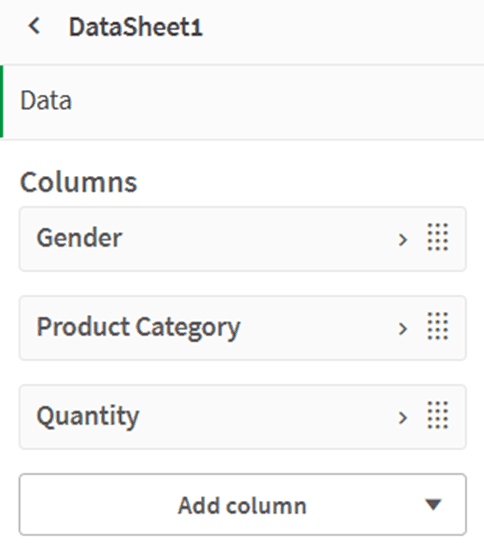
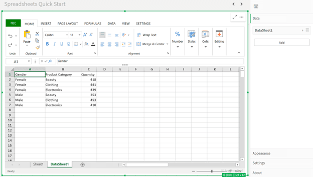
After completing these steps, your visualization will contain:
- One empty sheet: Sheet1
- One data-populated sheet from the Data Section: DataSheet1
Step 4: Format the Spreadsheet
- Remove the empty sheet:
- Right-click on Sheet1 and select Delete.
- Create a table on the remaining data sheet:
- Select all cells containing data.
- Go to the INSERT section in the Ribbon Menu.
- Click Table, then confirm in the pop-up window.
- Adjust formatting:
- Resize columns and rows as needed.
- Customize font styles using the HOME tab.
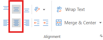
- Select your header cells and use alignment tools under Font Alignment.
Step 5: Add a Chart
- Select all cells containing data.
- Go to the INSERT tab in the Ribbon Menu.
- Click Insert Chart and choose a chart type that fits your data.
- Click OK.
Reposition your chart anywhere on the sheet.
Optional: Export Your Spreadsheet to Excel
If you want to continue working in another tool like Excel:
- Go to the FILE tab in the Ribbon Menu.
- Click Export .
- Select the Excel file option.
- Configure your export settings using Save Flags .
- Click the Export Excel File button.
- Name your file in the pop-up window and click OK.
After that, the download will start automatically, and your .xlsx file will be ready to open in Excel or any compatible software.
Use existing excel template
This guide walks you through how to use the AnyChart Spreadsheets extension in Qlik Sense to turn an Excel template into a fully interactive, data-driven spreadsheet.
Video walkthrough
Prerequisites
- Qlik Sense app with the AnyChart Spreadsheets extension installed
- Template file: personal-budget.xlsx
Step 1: Load Data into Qlik
- Upload the personal-budget.xlsx file to the Attached Files of your Qlik app.
- Open the Data Load Editor and use the following script to load the Budget and Transactions tables:
LOAD
Category,
Budget
FROM [lib://AttachedFiles/personal-budget.xlsx]
(ooxml, embedded labels, header is 3 lines, table is Budget)
Where Upper(Trim(Category)) <> 'TOTAL';
LOAD
"Date",
Description,
Category,
Amount
FROM [lib://AttachedFiles/personal-budget.xlsx]
(ooxml, embedded labels, header is 1 lines, table is Transactions); - Click Load Data.
Step 2: Add the Spreadsheets Extension
- Create a new sheet in your Qlik app and open it.
Enter Edit Mode. - From the Custom Objects > AnyChart section, drag the Spreadsheets Table visualization onto the canvas.
Step 3: Turn on Autosave
- Select the visualization and open the Properties Panel.
- Go to the Settings -> Autosave section
Step 4: Import the Excel Template
- With the visualization selected, go to the FILE tab in the ribbon menu.
- Click Import Excel File .
- Select the personal-budget.xlsx file.
The template contains two sheets:
- A Budget sheet
- A Transactions sheet
Step 5: Create Data Sections
- Open the Properties Panel and navigate to the Data tab.
- Click Add to create the first Data Section:
- Add dimension:
- Category
- Add measures:
- Sum(Budget)
- Sum(Amount)
- Sum(Budget) - Sum(Amount)
- Add dimension:
- Click Add again to create the second Data Section:
- Add dimensions:
- Date
- Description
- Category
- Add measure:
- Sum(Amount)
- Add dimensions:
- Customize measure labels (e.g., rename Sum(Amount) to Amount ).
Step 6: Prepare Template for Qlik Data
- Switch to each sheet in the spreadsheet view.
- Clear static cell values where Qlik data will be injected.
- Set those cells' format to General using the ribbon (this is important for formulas to work properly).
Step 7: Insert QLIK.DATA Formulas
Budget Sheet
- In the starting cell of the budget table (e.g., A4), enter:
=QLIK.DATA(0,,,TRUE,”TOP”)
This pulls data from the first Data Section and enables both labels and totals.
- Format data cells (e.g., Budget, Amount, and Difference columns) as Currency .
Transactions Sheet
- In the starting cell of the transactions table (e.g., A2 ), enter:
=QLIK.DATA(1,,,TRUE)
This uses the second Data Section and shows labels.
- Format the Date column as Short Date , and the Amount column as Currency .
Step 8: Final Formatting and Save
- Make any final formatting adjustments.
- Click the USER tab in the ribbon and select Save to app to store your changes.
Result
You now have a fully interactive spreadsheet that combines:
- A familiar Excel layout
- Live Qlik data
- Dynamic calculations using QLIK.DATA
Demos
Coming soon.
Sheets
The Spreadsheets extension supports working across multiple sheets—just like in Excel—enabling you to organize your data, calculations, and layouts across logical layers of a workbook.
Each sheet can contain a mix of:
- Static values — manually typed-in text or numbers.
- Functions — including references to other cells, ranges, or calculations.
- Data-linked cells — dynamically populated from Qlik data or QLIK formulas.
Sheets are fully independent:
- You can use different layouts and designs per sheet.
- Each sheet may display different hypercube data or none at all.
- The structure and formatting on one sheet will not interfere with another.
Sheet-to-Sheet References
Just like in Excel, you can reference cells from other sheets using the SheetName!CellReference format.
For example: =Sheet2!A1
This formula pulls the value from cell A1 on a sheet named Sheet2 .
This makes it easy to create summary sheets, aggregate values, or build dashboards that combine multiple sheet outputs.
You can rename sheets and rearrange their tabs freely, offering flexibility in how you design the workbook structure.
Data
The Spreadsheets extension introduces a data model that integrates Qlik’s associative engine with a flexible, Excel-like editing environment. This section covers how Qlik data is structured inside the extension and how it can be connected to spreadsheet content.
Data Sections
Data Sections define reusable datasets built from Qlik dimensions and measures. These act as the bridge between Qlik and the Spreadsheets canvas.
Data Sections Overview
- A Data Section consists of Columns, where each column is a Dimension or a Measure from Qlik.
- The order of Columns is customizable.
- Data Sections are managed from the Properties Panel of the Spreadsheets extension.
- Each Data Section can be reused across sheets or tables and supports multiple connection modes (see Connecting Data Sections ).
Totals
Each Data Section supports automatic totals per Measure columns:
- Enable totals from the Presentation tab of the Data Section configuration.
- Configure:
- Position: Top / Bottom / None
- Label: Customize text (e.g., "Total", "Summary")
Totals are calculated by Qlik and dynamically updated based on selections.
Columns
Each column in a Data Section represents either a Qlik dimension or measure, similar to fields in native Qlik tables. Columns are rendered in the spreadsheet to display actual values from the Qlik engine.
By default, columns are rendered in the order they are added — top to bottom — starting from the top-left corner of the sheet or the assigned data region.
Range
You can optionally specify a range for each column to control where exactly its values should appear in the sheet.
- Example (vertical): C1:C5 will place the column’s values into cells C1 through C5.
- Example (horizontal): C3:H3 will populate cells horizontally across row 3.
Only values that fit within the defined range will be shown. If more values exist than available cells, the column is automatically truncated.
Ensuring Data Ranges Fit Within the Sheet
When using custom ranges for columns — whether vertical (e.g., C1:C10) or horizontal (e.g., C3:H3) — it's important to make sure the spreadsheet has enough space to display the data.
The rendered data must fit within the current sheet range, which is defined by the number of visible rows and columns. If the specified column range exceeds these limits, some data may be cut off, fail to render correctly, or cause unexpected behavior.
Adjusting Sheet Dimensions
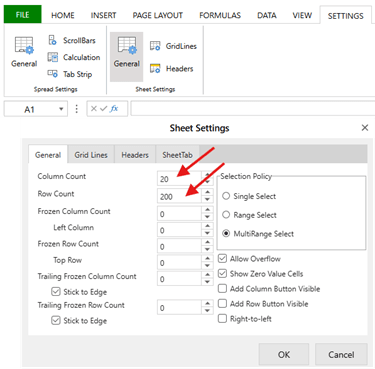
To avoid such issues:
- Go to the Settings tab in the Ribbon Menu.
- Select General under Sheet Settings.
- Increase the Row Count and/or Column Count as needed.
Known Behaviors and Limitations:
- Scrolling: Range settings may impact scroll behavior (see Scrolling section ).
- Offsets: If different columns have different start positions (e.g., A1, B5, C10), data loading and scrolling will align based on the first column’s offset.
- Mixed Offsets: Using non-uniform starting points (like A3, C5, E7) may result in gaps or unexpected rendering during data loading.
- Data Loading: The first-load and scroll-triggered loading always respect the offset of the first column when calculating how many rows to fetch
Connecting Data Sections
Once a Data Section is defined, you can connect it to your spreadsheet in three main ways:
Data Sections Overview
Each connection method offers a different balance of automation and control and suitable for different use cases, each having certain pros and cons:
| Method | Use Case | Control | Best For |
| Synced Sheet (default) | Auto-populate a new sheet with data | Low | Quick previews, one section/sheet |
| Table Binding | Link a Data Section to a spreadsheet table | Medium | Tabular data views, fixed layouts |
| QLIK Formulas | Insert data manually via formulas | High | Custom templates, advanced layouts |
Create Synced Sheet
- Enabled via the "Create Synced Sheet" toggle when adding a Data Section.
- Automatically creates a sheet named after the section label and injects the data.
- Suits for fast iteration and testing new data configurations.
🛈 Sheet is automatically updated if the Data Section changes.
Table Binding
Bind a Data Section directly to an existing table inside the spreadsheet.
Steps:
- Select a table in the spreadsheet view.
- Go to the Table Design tab in the Ribbon Menu.
- Open the Select Source dropdown.
- Select a Data Section.
The table will auto-populate with data from the selected section, with columns mapped in order.
This is ideal for pre-designed layouts or when you want to use Excel features like structured table formulas, formatting, or charts on live Qlik data.
QLIK Formulas
Power users can manually insert data using Qlik-aware formulas. These allow full control over layout and logic:
- QLIK.DATA() – inject data block
- QLIK.DATA.LABEL() – insert column labels
- QLIK.DATA.TOTAL() – insert total row values
In addition to the data-binding functions above, the QLIK.EXPRESSION() formula allows you to evaluate arbitrary Qlik expressions directly inside the spreadsheet — dynamically reflecting changes in Qlik selections.
🛈 Note: Since these formulas are powered by live Qlik data, updates in the Qlik app (e.g., filters, selections, or underlying data changes) will immediately affect the spreadsheet. This can result in the number of populated cells increasing or decreasing, so plan your layout accordingly.
For detailed syntax and examples, see Qlik-Related Functions section
Qlik Selections
If your Spreadsheet is built on Data Sections, it will dynamically respond to Qlik selections.
You can also perform Qlik selections directly from the Spreadsheet extension.
How to apply selection from the Spreadsheet
- Select the cells you want to filter.
- Right-click the selection.
- Choose Qlik Select from the context menu.
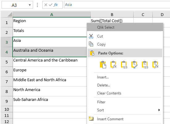
The Spreadsheets extension will automatically detect valid selections and apply them to the Qlik app.
Excel Functions
The extension supports most native Excel functions, including:
- Math & Trig: SUM, AVERAGE, ROUND, INT
- Logic: IF, AND, OR, NOT
- Text: CONCATENATE, LEFT, RIGHT, TEXTJOIN
- Lookup: VLOOKUP, INDEX, MATCH
- Date & Time: TODAY, NOW, DATEDIF, EOMONTH
- Array: UNIQUE, SORT, FILTER
And many others.
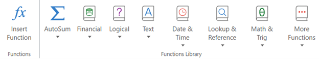
Feel free to explore a full list of available excel functions in the Formulas section of the Ribbon Menu
Qlik-Related Functions
The Spreadsheets extension supports a set of Qlik-specific formulas that allow you to interact with data sections, extract values, labels, totals, or evaluate expressions directly in spreadsheet cells.
Each function runs asynchronously and returns dynamic values based on Qlik's associative model.
QLIK.DATA
Fetches and inserts data values from a preconfigured Data Section.
= QLIK.DATA(data_section_label_or_index, [column_label_or_index], [is_horizontal], [show_label], [show_total], [limit])
Arguments:
- data_section_label_or_index – Label or index of the Data Section.
- column_label_or_index – (Optional) Label or index of the column (dimension or measure).
- is_horizontal – (Optional) If true, data fills horizontally instead of vertically.
- show_label – (Optional) If true, includes column labels.
- totals_position – (Optional, Enum) Controls if and where total values are inserted.
- "INHERIT" – Use total settings defined in the Qlik panel (definition section).
- "TOP" – Insert total values above the data range.
- "BOTTOM" – Insert total values below the data range.
- "NONE" (default) – No totals are inserted.
- 🛈 Invalid values will be treated as "NONE".
- limit – (Optional) Sets the maximum number of rows (or columns, if horizontal) to return from the Data Section. This is not the same as setting limitations in the Data Section, this is a hard limit on the number of rows, please use Data Section limitation if you need proper limitation on measure.
Use cases:
- Embedding Qlik data into specific spreadsheet regions.
- Populating sheets with multiple datasets independently.
- Displaying data when automatic sheet-to-section binding is not desired.
QLIK.DATA.LABEL
Returns the label of a specific dimension or measure from a Data Section.
=QLIK.DATA.LABEL(data_section_label_or_index, column_label_or_index)
Arguments:
- data_section_label_or_index – Label or index of the Data Section.
- column_label_or_index – Label or index of the dimension or measure.
Use cases:
- Dynamically showing column headers.
- Building generic or reusable templates with flexible data inputs.
QLIK.DATA.TOTAL
Returns the total aggregation value for a specific measure in a Data Section.
=QLIK.DATA.TOTAL(data_section_label_or_index, column_label_or_index)
Arguments:
- data_section_label_or_index – Label or index of the Data Section.
- column_label_or_index – Label or index of the column .
Use cases:
- Displaying total rows or summary KPIs outside the main data block.
- Referencing Qlik-calculated totals without manual summing.
QLIK.EXPRESSION
Evaluates a Qlik expression and returns the result.
=QLIK.EXPRESSION("=Today()")
Arguments:
- query_string – A Qlik expression wrapped in quotes (must start with =).
Use cases:
- Display aggregated measures (KPI)
=QLIK.EXPRESSION("=Sum(Sales)")- Combine with spreadsheet features like conditional formatting to highlight:
- Green if above target
- Red if below
- Display applied selections
=QLIK.EXPRESSION("=GetSelectedCount(Country)")=QLIK.EXPRESSION("=GetFieldSelections(Region, ' | ')")
- Display system values
=QLIK.EXPRESSION("=Now()")=QLIK.EXPRESSION("=OSUser()")=QLIK.EXPRESSION("ReloadTime()")
Live Expression Evaluation
All values returned by QLIK.EXPRESSION() are dynamic and update in real time based on:
- Selections made in the Qlik app
- Underlying data changes
- System or session context
These values can change between sessions or users — ideal for live dashboards or personal views.
Tip: Use this function alongside native Excel logic (IF, TEXT, ROUND, etc.) to create smart dashboards directly inside the spreadsheet.
Practical Examples
KPI
It is possible to build KPIs based on Qlik formulas and then apply conditional formatting rules to highlight results visually.
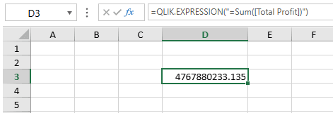
1. Insert KPI Formula
Enter a Qlik expression into a cell. For example, to calculate the total profit:
=QLIK.EXPRESSION("Sum([Total Profit])")
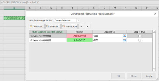
2. Apply Conditional Formatting
Use Spreadsheet’s Conditional Formatting feature to dynamically style the cell based on the KPI result.
Example rules:
- Green if Total Profit is greater than 2,400,000,000
- Red if Total Profit is less than 2,400,000,000
3. Live Updates
When selections are applied in Qlik, the KPI value will automatically update, and formatting will be re-evaluated in real time.
This makes it easy to build live KPI dashboards where visual indicators instantly respond to Qlik filters and selections.
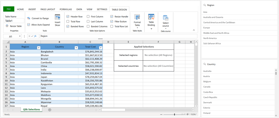
Selection Status Banner
A Selection Status Banner allows you to show which values are currently selected in the Qlik app. This makes it easy to provide context inside your spreadsheet reports, ensuring that end users always know which filters are active.
Unlike simple KPIs, here we are using more complex Qlik formulas that combine multiple functions ( IF, GetSelectedCount(), GetFieldSelections() ). This demonstrates that you are not limited to basic expressions — it is possible to construct flexible formulas to match your exact reporting needs.
1. Insert Selection Formulas
To show the selected Region: =QLIK.EXPRESSION("=IF(GetSelectedCount(Region) = 0, 'No selection (All Regions)', GetFieldSelections(Region, ' | '))")
To show the selected Country: =QLIK.EXPRESSION("=IF(GetSelectedCount(Country) = 0, 'No selection (All Countries)', GetFieldSelections(Country, ' | '))")
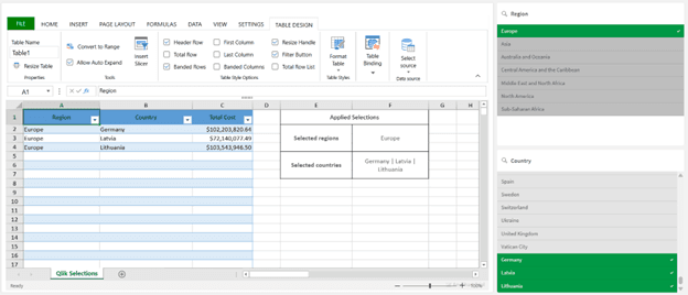
2. Result with Active Selections
When the user applies selections in the Qlik app, the banner automatically updates to reflect the chosen values.
If Europe is selected in Region → the cell shows Europe.
If Germany, Latvia, Lithuania are selected in Country → the cell shows Germany | Latvia | Lithuania.
This example uses an IF wrapper to handle the “No selection” case, but you can adapt the logic:
- Replace text strings with your own wording ("All Regions" → "All Values").
- Concatenate multiple fields into one line (e.g., Region + Year).
- Apply conditional formatting to highlight when filters are too narrow or too broad.
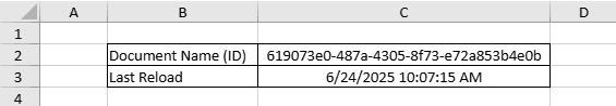
App & System Meta (Live)
It is possible to display application metadata directly in the spreadsheet using Qlik system functions. This ensures that every report clearly communicates which app it came from and when the data was last refreshed.
1. Insert Metadata Formulas
Document name:
=QLIK.EXPRESSION("=DocumentName()")
Reload timestamp:
=QLIK.EXPRESSION("=ReloadTime()")
Formatting
The Spreadsheets extension offers a comprehensive suite of formatting tools available in the Ribbon Panel, organized by sections. Below are the most frequently used tools from the Home tab, helping you quickly style and structure your spreadsheet content.
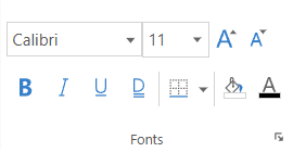
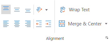
Home
- Fonts : font size, color, bold, italic, underline, background fill, borders
- Text Aligning : Vertical and horizontal alignment, Orientation, Indent, Wrap, Merge and Center
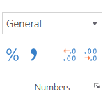
- Number formats : currency, percentage, custom formats
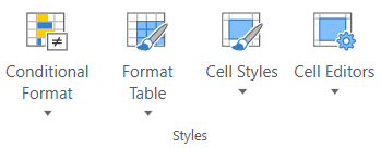
- Cell Styling : Conditional Format, Table Format, Cell Styles, Cell Editors
- Cells : Insert, Delete, Format

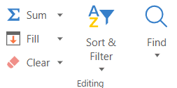
- Editing : Insert Function, Fill, Clear, Sort and Filter, Find
Scrolling
The Spreadsheets extension implements vertical scrolling to support smooth interaction with large datasets, especially when using Qlik-connected Data Sections. This behavior is automatic and depends on the sheet type and how data is connected.
This section describes how scrolling affects data loading and rendering, and outlines important details for advanced use cases.
Scrolling General
- As the user scrolls vertically and approaches the bottom of the visible area, the system checks whether more rows should be added or data should be loaded.
- Horizontal scrolling is supported for navigation only and does not trigger data loading or range expansion.
Synced Data Sheets
When using the Create Synced Sheet for the Data Section , the spreadsheet will automatically handle large datasets by loading more rows as you scroll.
As you move down the sheet, if more Qlik data is available, it will seamlessly appear below the visible rows — no need to manually trigger or reload anything. This makes working with long tables feel fluid and uninterrupted.
If there’s no more data left to load, the sheet will still let you scroll further, but the new rows will appear empty.
This behavior ensures:
- You never hit a hard stop while scrolling.
- New data appears only when needed.
- Layout remains consistent, even when reaching the end of the data.
You can control how much data is loaded initially by adjusting the Rows Count setting in the sheet’s settings.
On Other Sheets
Sheets that are not linked to Data Sections through Create Synced Sheet do not trigger any automatic row addition or data loading during scrolling.
Range Offset and Data Loading
The system respects the range offset of the first column in a Data Section when calculating data loading behavior.
- If the first column's range starts at a lower row (e.g., A100), the sheet begins rendering from that position.
- All scrolling and data fetching logic is based on that first-column offset.
Limitations and Edge Cases
- Horizontal ranges (e.g., A1:Z1) will render data correctly for the first set of values but will not support additional data loading during vertical scrolling. The user must manage layout and visibility manually in such cases.
- Mixed column offsets (e.g., A1, B5, C10) may result in:
- Inconsistent alignment
- Gaps in the displayed data
- Data appearing only partially loaded
Data fetching is always aligned with the first column's offset, regardless of how other columns are configured.
Performance Considerations
Custom ranges with large offsets or very high row counts can significantly increase data volume during load.
For example:
- A Data Section with 5 columns and a user-defined row limit of 10,000 will attempt to load and render 50,000 cells.
- This may affect performance, especially in older browsers or lower-end machines.
To maintain responsiveness, consider:
- Limiting the number of rows where possible.
- Avoiding unnecessarily large starting offsets.
Open / Save
The Open / Save functionality in the File Menu allows you to preserve, reuse, and share the content of your Spreadsheet.
You can choose from 2 storage locations for saving and loading your Spreadsheet configurations. Each option can be enabled or disabled in the Properties Panel. Once enabled, the corresponding section will appear in the File Menu.
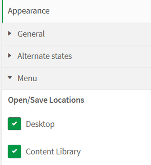
Option 1: Desktop
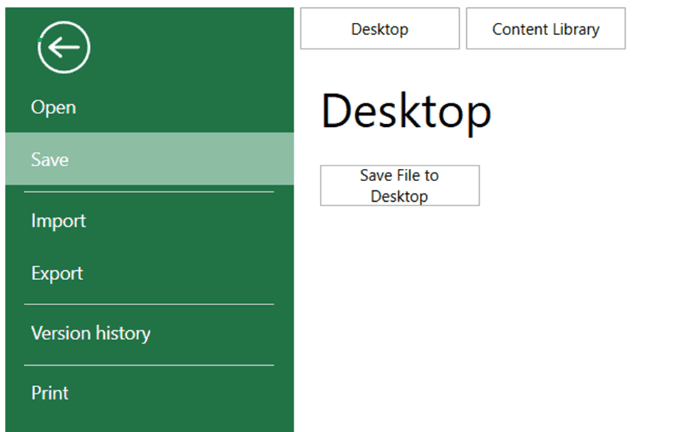
- Saves your Spreadsheet configuration as a JSON file on your computer.
- Best for sharing directly with individual users or keeping private copies.
To open a saved file:
- Go to the File Menu → Open → Desktop.
- Click Select File.
- Choose the previously saved JSON configuration file.
Option 2: Content Library
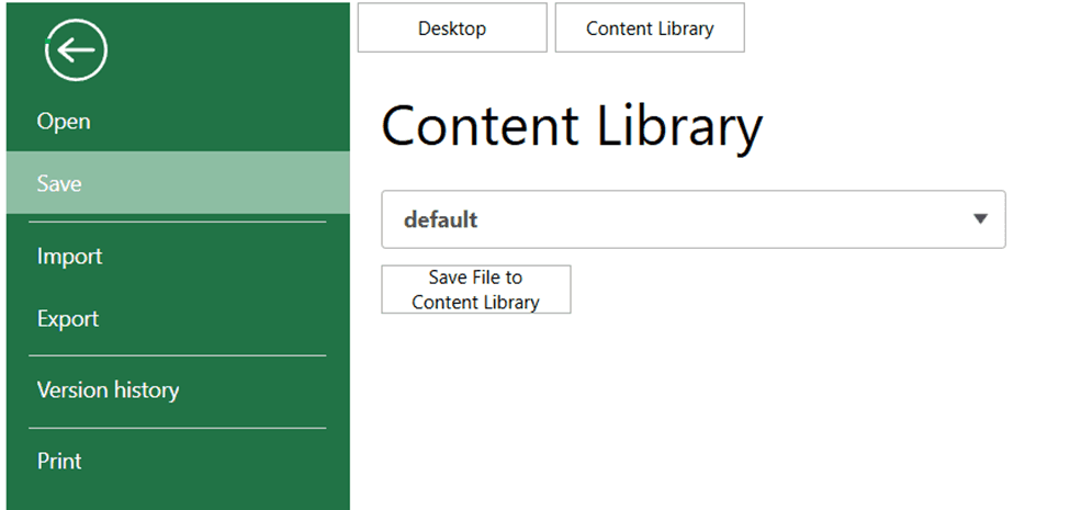
- Saves your configuration as a JSON file inside the chosen Qlik Content Library.
- Similar to the Desktop option, but the file is stored in Qlik rather than locally.
- Best for maintaining multiple versions of Spreadsheet setups accessible to all users with Content Library access.
Tip: For temporary changes that don’t need saving, use the Autosave functionality.
Autosave
The Autosave functionality lets you preserve changes in your Spreadsheet without explicitly saving them to a stable configuration.
When enabled, any change you make is automatically recorded after 3 seconds of inactivity. These autosaved changes are stored locally in your browser and are only available to you (not shared with other users).
There are three storage options:
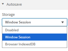
Option 1: Window Session
- Saves the current configuration in your browser session.
- Changes remain available as long as the browser window stays open.
- Closing the browser will discard all autosaved changes.
Option 2: Browser IndexDB
- Saves the current configuration in the browser’s IndexedDB storage.
- Changes are preserved even after closing and reopening the browser.
- Best for keeping your personal work-in-progress across multiple sessions.
Option 3: Disabled
- Completely turns off Autosave.
- No changes are preserved automatically.
Note: Use Window Session for temporary work, IndexedDB for persistent personal drafts, or Disabled if you only want manual saves. At the same time, it is not recommended to store impactful changes long-term with Autosave. Consider using the stable saving options for long-term changes.
Version History
When the Autosave functionality is enabled, the Version History option becomes available in the File Menu.
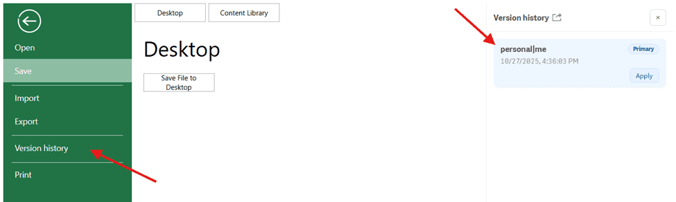
Version History allows you to access the latest autosaved versions of all authorized users who have access to the application.
In other words, when users make changes to the Spreadsheet, their most recent autosaved versions will appear in the Version History tab — making it easy to review and restore them.
You can browse each saved version to inspect its contents.
Click Apply to restore a selected version as your current Spreadsheet state.
- If you are not the owner of the Qlik application, the applied version will affect only your personal last saved version of the Spreadsheet.
- If you are the owner of the application, applying a version will update the default configuration of the Spreadsheet for all users.
Import / Export
The Spreadsheets extension provides robust tools for importing and exporting data, enabling smooth interaction with external files and software
Importing Excel or CSV Files
To import data, open the FILE tab in the ribbon menu and select Import. You can upload either an .XLSX (Excel) or .CSV file.
Each import type includes a set of configurable options that control how the file is processed. Depending on the selected format, you may be able to preserve formatting, formulas, merged cells, calculation settings, and more. These options ensure that imported content behaves and appears as expected in the Qlik environment.
Once imported, the spreadsheet maintains its structure and styling, making it easy to continue working with existing data or templates. You can also enrich the imported file with Qlik-driven charts, additional sheets, or calculated logic.
Exporting to Excel, CSV, or PDF
To export your spreadsheet, go to the FILE tab and choose Export. You can save the current workbook in .XLSX, .CSV, or .PDF format, depending on your needs.
Each export format includes its own configuration panel, allowing you to tailor the output. For example, you may choose to include styles, formulas, layout elements, headers, or control how merged and empty cells are handled. These options help ensure your exported document preserves the desired structure and content fidelity.
Note: when exporting to Excel, make sure the “ Include Binding Source ” flag is turned on. Otherwise the export may be corrupted.
Writeback
The Spreadsheets extension allows you not only to work with data already loaded into a Qlik app, but also to write new or updated data back to an external database. This capability enables interactive, operational use cases where users can edit data directly in a spreadsheet-like interface and persist those changes outside of Qlik.
The Writeback functionality exists specifically to support this workflow. In this section of the documentation, you will learn how to set up an environment for writeback, connect the Spreadsheet extension to a backend service, and effectively use writeback features in your Qlik apps - from configuring data connections to editing data and reloading app content.
Overview
How Writeback Is Structured
1. Data Config - defining data connections
In Data Config, you configure how the Spreadsheet extension connects to your backend:
- Define HTTP endpoints for reading and writing data (GET, POST, PUT, DELETE, BATCH).
- Configure authentication (optional).
- Create logical Tables that describe how a database table is accessed.
A Table in this context is a configuration object that represents:
- a backend endpoint,
- a database table or view,
- and the rules for interacting with it.
2. TableSheet - editing data
In TableSheet, you select one of the configured Tables and bind it to the sheet.
Once connected:
- Data is loaded from the backend.
- The TableSheet displays a table view that represents the database data.
Users can:
- edit cell values,
- add new rows,
- delete existing rows.
All changes are performed directly in the spreadsheet-like UI.
Under the hood, these actions translate into CRUD or batch requests sent to the backend.
3. Saving changes and reloading data
When users finish editing data:
- Changes are sent to the backend and persisted in the database.
- The Qlik app itself is not automatically updated.
- To see updated data in Qlik visuals, the user explicitly triggers a reload.
Two reload options are available:
- Partial Reload
Refreshes data for the current user session. - Full Reload
Reloads the full application data model (available to power users only).
Reloads are triggered via the Qlik Engine API and depend on the app’s load script being configured correctly to read updated data from the backend.
Backend for Writeback
To support writeback, we provide a sample reference backend built with:
- Node.js
- Express
- SQLite
GitHub repository with a sample backend solution: https://github.com/AnyChart/writeback-server-example
This backend:
- Implements the required CRUD and batch endpoints.
- Stores data in a relational database.
- Demonstrates how writeback integration works end to end.
The provided backend is demonstrational:
- It is suitable for local testing and demos.
- It is intended as a reference implementation.
- Users are expected to adapt or replace it with their own backend for production use.
What Writeback Is (and Is Not)
Writeback is:
- explicit - users decide when to save and reload,
- controlled - no background or scheduled reloads,
- flexible - works with both demo and custom backends.
Writeback is not:
- providing real-time synchronization,
- providing automatic background refresh,
- a replacement for backend data governance.
Typical Writeback Flow
- Configure backend connections in Data Config.
- Bind a configured Table to TableSheet.
- Edit data directly in the TableSheet.
- Changes are sent to the backend and saved.
- Trigger Partial or Full Reload to refresh Qlik data.
Edit → Save → Reload → See updated data in Qlik
________________________________________
Quick Start
This section shows the fastest way to get a working writeback demo using the provided reference backend.
This guide focuses on the happy path and avoids advanced topics such as custom backends, paging, or complex validation.
Prerequisites
- Qlik Sense Desktop
- The Spreadsheet extension is already installed.
- Node.js
- Basic familiarity with:
- Qlik load scripts
- Adding objects to a Qlik sheet
Note: The same workflow applies to other Qlik platforms.
Video Tutorial
Coming Soon
Step 1: Start the Demo Writeback Backend
We provide a sample reference backend built with Node.js + Express + SQLite.
It can be adapted to your real-life environment.
- Clone the repository:
git clone https://github.com/AnyChart/writeback-server-example
cd writeback-server - Install dependencies:
npm install - Configure environment variables
Create a .env file and set following variables:
PORT = 3333
TOKEN = testtoken123 - Start the server:
npm start - Verify the backend is running:
a. Open a browser or REST client
b. Check that the GET endpoint responds
http://localhost:<PORT>/employees/get
At this point, the backend and demo database are running locally.
Step 2: Create a REST Connector in the Qlik App
To make writeback changes visible in Qlik visualizations, the app must load data directly from the backend.
This is done using a REST connector.
- Open the Data Load Editor.
- Create a new REST connector.
- Set the backend GET endpoint URL (for example, http://localhost:3333/employees/get).
Authentication (Important)
If your backend requires authentication (as in the demo backend):
Add a custom header to the connector:
Name: Authorization
Value: Bearer YOUR_TOKEN
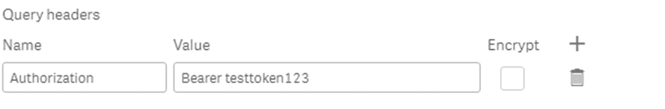
Notes:
- The token value must match the token used in the Spreadsheets extension.
- If your backend does not require authentication, this header can be omitted.
- Authentication handling depends entirely on your backend implementation.
Save the connector.
In this example, the connector is named Writeback_DEMO
Step 3: Add a Load Script to Read Data from the Backend
After creating the REST connector, add a load script that reads data from it.
Example load script:
LIB CONNECT TO 'Writeback_DEMO';
RestConnectorMasterTable:
SQL SELECT
 "id",
 "Region",
 "Director",
 "Salary",
 "HiredDate",
 "FiredDate"
FROM JSON (wrap on) "root";
[employees]:
REPLACE LOAD
 [id],
 [Region],
 [Director],
 [Salary],
 [HiredDate],
 [FiredDate]
RESIDENT RestConnectorMasterTable;
DROP TABLE RestConnectorMasterTable;
Reloads (Partial or Full) re-run this script to reflect writeback changes.
Step 4: Add the Spreadsheet Extension to the App
- Open your Qlik app.
- Add the Spreadsheet object to a sheet.
At this point, the spreadsheet is visible but not yet connected to any data source.
Step 5: Configure a Data Source (Data Config)
- Open Data Config inside the Spreadsheet extension.
- Create a new Table.
- Enter backend authentication credentials (token).
- Configure the backend endpoints (example: employees table):
- GET: http://localhost:3333/employees/get
- POST: http://localhost:3333/employees/post
- PUT: http://localhost:3333/employees/put
- DELETE: http://localhost:3333/employees/delete
- BATCH: http://localhost:3333/employees/batch
- Save the configuration.
This step defines how the Spreadsheet extension communicates with the backend.
Step 6: Bind the Table to TableSheet
- Switch to TableSheet.
- Select the configured Table from the list.
- Bind it to the sheet.
Once bound:
- Data is loaded from the backend.
- A table view representing the database is displayed.
- Cells become editable.
Step 7: Test Writeback
- Edit an existing value in TableSheet or add a new row.
- Save/apply changes.
- Trigger a reload:
- Partial Reload (recommended)
- Full Reload (also available)
The extension will:
- send changes to the backend,
- persist them in the database,
- reload the app via the Qlik Engine API.
Step 8: Verify the Result
After the reload completes:
- The updated data should appear:
- in other Qlik visualizations (e.g. tables, KPIs),
- not just inside the Spreadsheet.
- This confirms that:
- writeback worked,
- data was saved,
- reload succeeded,
- the load script is reading updated data.
Data edited in TableSheet → saved to database → visible in Qlik visuals.
________________________________________
Architecture
This section describes the architecture of the Writeback functionality in the Spreadsheets extension and how its main components interact with each other.
High-Level Flow
At a high level, the writeback architecture follows a client-driven, explicit interaction model:
- The user edits data in the Spreadsheets extension.
- The extension sends writeback requests to a Writeback Backend.
- The backend persists changes in a database.
- The user explicitly triggers a reload from the extension.
- The Qlik app reloads data and updates visualizations.
There is no background synchronization and no automatic reload after writeback.
All state changes are initiated by user actions.
Main Components
Data Config (Extension)
Data Config is the configuration layer inside the extension.
Responsibilities:
- Define Tables and their backend endpoints for:
- GET
- POST
- PUT
- DELETE
- BATCH
- COLUMNS
- Configure authentication.
A Table is a configuration object, not data itself.
It describes how the extension communicates with the backend.
TableSheet (Extension)
TableSheet is the data interaction layer.
Responsibilities:
- Bind a configured Table to a dedicated view (TableSheet).
- Display backend data in a tabular format.
- Allow users to:
- edit cell values,
- add rows,
- delete rows,
- perform reload
- Collect changes and prepare them for writeback.
TableSheet represents the current data state loaded from the backend, not a cached or authoritative copy.
Writeback Backend
The Writeback Backend is an HTTP service responsible for data persistence.
Responsibilities:
- Accept CRUD and batch requests from the extension.
- Process incoming data (as defined by the backend implementation).
- Persist data in a database.
- Return updated rows or operation results.
Important boundaries:
- The backend is agnostic of Qlik.
- The backend does not trigger reloads.
- The backend does not manage user sessions inside Qlik.
The provided Node.js + Express + SQLite backend serves as a reference implementation, intended to be adapted or replaced in production environments.
Database
The database stores the authoritative state of the data.
Key characteristics:
- The backend is the single source of truth.
- Changes are applied immediately on writeback requests.
- There is no intermediate staging layer.
Multi-user behavior follows a last-write-wins model:
- Concurrent updates are resolved by order of execution.
- No locking or merge logic is applied.
This approach avoids conflicts by definition and keeps the system predictable.
Qlik App and Engine
The Qlik App loads data from the backend via its load script.
Responsibilities:
- Fetch data from the backend using GET endpoints.
- Build the app’s data model.
- Update visualizations after reload.
Reloads are triggered from the Spreadsheets extension using the Qlik Engine API.
There are:
- no QMC reload tasks,
- no scheduled reloads,
- no server-initiated reloads.
Authentication
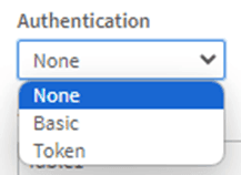
Authentication between the Spreadsheets extension and the writeback backend supports three modes:
- None — requests are sent without any authentication data.
- Basic — requests include a username and password.
- Token — requests include a Bearer token in the Authorization header.
The extension only attaches the selected authentication data to outgoing requests.
The exact authorization logic, validation rules, and access control are fully governed by the backend.
Authentication is optional and depends on backend requirements.
Reload Model in Architecture
Reload logic is fully owned by the Spreadsheets extension (not backend).
- Reloads are triggered explicitly by the user.
- Partial and Full reloads are supported.
- Reloads use the Qlik Engine API only.
Reload is a separate step from writeback and is never automatic.
Architecture Summary
The writeback architecture is intentionally simple and explicit:
- UI and interaction live in the Spreadsheets extension.
- Persistence is handled by a backend service.
- Data reload is user-driven and session-aware.
- Multi-user behavior is deterministic via last-write-wins.
- No QMC, no reload tasks, no background processes.
This design keeps responsibilities clearly separated and allows the solution to scale from demos to production environments without architectural rewrites.
________________________________________
Backend Setup
Purpose of the Writeback Backend
The Writeback backend is a required component that persists data changes made in the Spreadsheets extension.
Its responsibilities include:
- accepting writeback requests from the extension,
- writing data to a database,
- returning updated records to the client.
The backend is intentionally decoupled from Qlik and does not manage reloads, sessions, or UI logic.
Demo Backend (Reference Implementation)
We provide a demo backend built with:
- Node.js
- Express
- SQLite
This backend serves as:
- a ready-to-run demo for local testing,
- a reference implementation for building your own backend.
It demonstrates:
- required CRUD and batch endpoints,
- expected request and response formats,
- basic authentication handling,
- database interaction patterns.
The demo backend is not production-grade and is intended for demonstration and learning purposes.
Running the Demo Backend
Detailed instructions for running and configuring the demo backend are maintained in the GitHub repository:
Writeback Server Repository - https://github.com/AnyChart/writeback-server-example
The repository README covers:
- installation steps,
- environment variables,
- authentication setup,
- database schema,
- available endpoints,
- example requests.
Using Your Own Backend
You are not required to use the demo backend.
Any backend implementation can be used, as long as it:
- exposes compatible CRUD and batch endpoints,
- accepts and returns JSON data,
- persists changes reliably,
- enforces authentication and validation as needed.
Responsibility for:
- data validation,
- security,
- access control,
- scalability
lies on the backend implementation.
The CRUD endpoints have to follow the next requirements:
Operation | Request Type | Request Data | Response Data |
update | POST | The updated data | The updated data |
read | GET | No data | The records array |
delete | DELETE | The deleted data or data array | No restrictions |
create | POST | The inserted data | The inserted data |
getColumns | GET |
| A column array, where each column contains the properties: The 'field' property is the name of the column. The 'dataType' property is the data type of the column. The 'defaultValue' property is the default value of the record in the column. The 'isPrimaryKey' property is the primary column. |
batch | POST | An object array, where each object contains a 'type' property. This operation type could be 'update', 'insert', 'delete', 'addColumn', 'updateColumn' or 'removeColumn'. The 'dataItem' property is the current record. The 'sourceIndex' property is the record index. The optional 'oldDataItem' property is the original record. The optional 'column' property is the current column. The optional 'data' property is the default value of the current added column. The optional 'originalColumn' property is the original column. For example: [ {"type":"addColumn","column":{...}}, {"type":"updateColumn","column":{...}, "originalColumn":{...}}, {"type":"removeColumn","column":{...}}, {"type":"delete","dataItem":{...}, "sourceIndex":5}, {"type":"insert","dataItem":{...}, "sourceIndex":3}, {"type":"update","dataItem":{...}, "oldDataItem":{...}, "oldDataItem":{...}, "sourceIndex":1}] | An object array, where each object contains a 'succeed' property which indicates an operation's success or failure, and an optional 'data' property, which is the current record and only for the 'insert' operation. For example: [{"succeed":true}, {"succeed":false}, {"succeed": true}, {"succeed":true}, {"succeed":false}, {"succeed": true}] |
Backend Summary
- The backend is mandatory for writeback.
- A demo backend is provided for convenience and reference.
- Production deployments should use a custom backend.
- Backend implementation details are documented in GitHub.
________________________________________
Extension Configuration
This section focuses on configuring the Spreadsheets extension inside a Qlik app so that it can communicate with a writeback backend, save data changes, and trigger reloads.
Data Source Configuration Overview
Writeback configuration is managed through the Data Source window.
In this window, you define one or more Tables, where each Table represents a logical connection to backend endpoints.
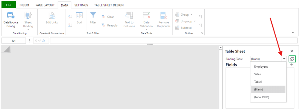
To access it, select the Data section in the Ribbon menu, and click Data Source Config button.
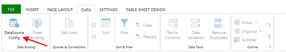
Table Settings
Authentication
Each Table can be configured with an authentication method.
The selected method is applied to all requests made for that Table.
Available options:
- None
No authentication is used.
Requests are sent without any authorization headers. - Basic
Uses a username and password pair.
Credentials are sent using standard HTTP Basic Authentication. - Token
Uses a Bearer token.
The token is attached to requests as an Authorization: Bearer <token> header..
Authentication is optional and depends entirely on how the backend is implemented.
Demo backend note:
The demo writeback server provided by AnyChart uses Token-based authentication by default. This is done for simplicity and clarity in the reference implementation.
Table Name
A logical name used inside the extension.
This name is later selected when binding the Table to a TableSheet.
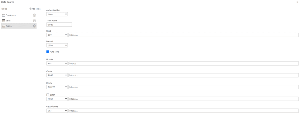
Endpoint Configuration
For each operation, specify:
- HTTP method
- Full endpoint URL
Supported operations:
- Read (GET)
Loads data into the TableSheet. - Create (POST)
Inserts new rows. - Update (PUT)
Updates existing rows. - Delete (DELETE)
Deletes rows. - Batch (POST)
Applies multiple create/update/delete operations in a single request. - Get Columns (GET)
Retrieves column metadata from the backend.
Notes:
- The Read (GET) endpoint is required to display data.
- Writeback actions only work if the corresponding endpoints are configured.
- If an endpoint is missing, the related action will not work correctly.
Binding a Table to TableSheet
After configuring a Table:
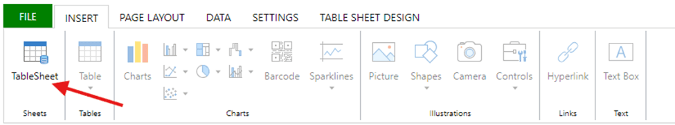
- Switch to TableSheet view, by selecting the Insert section in the ribbon menu, and clicking the TableSheet button.
- Select one of the configured Tables from the dropdown.
- Observe bounded table on the TableSheet
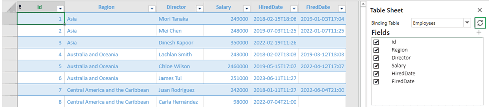
Once bound, the TableSheet displays data returned by the Read endpoint and allows editing according to the configured operations.
________________________________________
Writeback Usage
This section explains how to work with writeback inside the Qlik app, using the TableSheet interface.
Editing Existing Rows
To edit existing data, first enable Row Action mode:
- Open the Table Sheet Design section in the ribbon menu.
- Click the Row Action button.
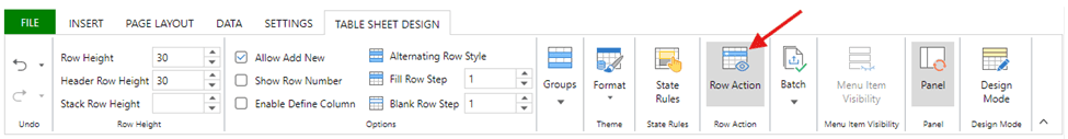
Once Row Action mode is enabled:
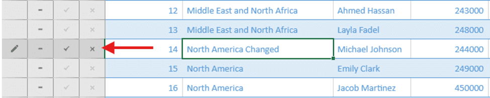
- You can edit values in any non-primary key column.
- Primary key columns are read-only and cannot be changed.
To save changes for a row:
- Click the checkmark (✓) icon on the left side of the row.
This action immediately sends an Update request to the backend.
To discard changes:
- Click the cross (✕) icon — the row is reverted to its previous state.
Adding New Rows
To add a new row:
- Scroll to the bottom of the TableSheet.
- Populate the last empty row with new data (at least one cell in the row must be filled).
If additional fields are required, this is defined by the backend schema.
To save the new row:
- Click the checkmark (✓) icon on the left.
- This sends a Create request to the backend.

If the backend allows missing or empty values, they are saved as-is.
Validation rules depend on how the backend is implemented.

Deleting Rows
To delete a row:
- Locate the row you want to remove.
- Click the minus (–) icon on the left side of the row.
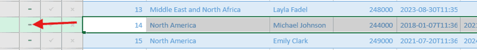
This action sends a Delete request to the backend.
Saving Changes and Batch Actions
Row-level actions (checkmark / minus icons) apply changes immediately for that row.
If you make changes to multiple rows and want to apply them together:
- Open Table Sheet Design in the ribbon menu.
- Open the Batch dropdown.
- Click Submit.
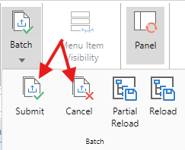
This sends all pending changes in a single batch request.
Note: to enable Batch functionality - Toggle on “Batch” option in the Data Source Config.
Reloading Data in Qlik
After making changes, reload the app to update other visualizations.
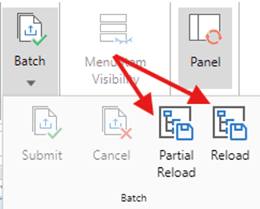
Reload controls are located in:
Ribbon menu → Table Sheet Design → Batch dropdown
Available options:
- Partial Reload
- Full Reload
Notes:
- Reloads are always triggered manually.
- Partial reload requires the app’s Load Script to be structured accordingly.
- When the reload finishes, all charts and tables in the app reflect the updated data.
Typical Workflow Example
A common writeback workflow looks like this:
- Edit values in the TableSheet
- Save rows using the checkmark
- Trigger Partial Reload
- See updated data in charts and tables
This keeps writeback explicit, predictable, and easy to control
AI Formula
The AI Formula feature allows you to run natural language queries using a connected AI model (in alpha version supports connection only with OpenAI). This enables spreadsheets to become interactive, intelligent tools — capable of generating or transforming content on the fly using language-based prompts.
Configuration (Property Panel)
To use AI formulas, go to the AI Formula section in the properties panel of the extension and configure the following settings:
- AI server URL
The endpoint for the OpenAI API (e.g., https://api.openai.com/v1/chat/completions) - AI model
Currently supports:- Gpt-3.5-turbo
- Gpt-4
(Additional models will be added in the future)
- Max tokens per request
Controls the length of the AI's response (default: 4000) - Formula evaluation mode
Determines when the AI is queried:- On recalculation
- Once
- On interval
- API Key
Your OpenAI secret key (must have valid access rights to the selected model)
Using the AI() Formula in the Spreadsheet
Once the above settings are configured, you can use the following formula directly in spreadsheet cells:
=AI("Translate this sentence to Spanish: " & A2)
Formula Syntax:
AI(query_string)
- query_string – A string prompt that will be sent to the selected model (can be static or dynamic using cell references)
The result will be displayed directly in the cell where the formula is entered.
Conversion from table extension
You can convert a standard Qlik Table chart into the Spreadsheets extension.
- All configured Columns from the original Table are automatically transferred into the default Data Section of the Spreadsheet.
- A corresponding sheet is created, containing all the same columns as the original Table.
How to convert a Table chart:
- Make sure you have a Table chart with data on the sheet of your app.
- Enter Edit Mode and open the Assets panel.
- Go to Custom Objects.
- Find the Spreadsheets extension.
- Drag and drop it onto the existing Table chart.
- Select Convert.
Note: Conversion works only one way. Converting a Spreadsheet back into a standard Qlik Table chart is not supported.
Tip: Use this feature to quickly migrate existing tables into Spreadsheets and unlock advanced editing and interaction features.
Hotkeys
The list of hotkeys available to usage with the Spreadsheet extension.
| KEY | ACTION |
| Ctrl+Z | undo |
| Ctrl+Y | redo |
| Ctrl + Down | navigationBottom |
| Down | navigationDown |
| End | navigationEnd |
| Ctrl+Right | navigationEnd |
| Ctrl+Home | goToSheetBeginning |
| Home | navigationHome |
| Ctrl+Left | navigationHome2 |
| Ctrl+End | goToSheetBottomRight |
| Left | navigationLeft |
| Tab | moveToNextCell |
| PageDown | navigationPageDown |
| PageUp | navigationPageUp |
| Ctrl+PageUp | NavigationPreviousSheet |
| Ctrl+PageDown | NavigationNextSheet |
| Shift+Tab | moveToPreviousCell |
| Right | navigationRight |
| Ctrl+Up | navigationTop |
| Up | navigationUp |
| Delete | clear |
| Back | clearAndEditing |
| Enter | commitInputNavigationDown |
| Shift+Enter | commitInputNavigationUp |
| ESC | cancelInput |
| Shift+Left | selectionLeft |
| Shift+Right | selectionRight |
| Shift+Up | selectionUp |
| Shift+Down | selectionDown |
| Shift+Home | selectionHome |
| Ctrl+Shift+Left | selectionHome |
| Shift+End | selectionEnd |
| Ctrl+Shift+Right | selectionEnd |
| Shift+PageUp | selectionPageUp |
| Shift+PageDown | selectionPageDown |
| Ctrl+Shift+Up | selectionTop |
| Ctrl+Shift+Down | selectionBottom |
| Ctrl+Shift+Home | selectionFirst |
| Ctrl+Shift+End | selectionLast |
| Ctrl+C | Copy |
| Ctrl+X | Cut |
| Ctrl+V | Paste |
| Alt+Enter | InputNewLine |